
A Beginners Guide to Beating the Bookmakers with TensorFlow
Alan - It says here we should use TensorFlow. Apparently we can use a Deep Neural Network to predict the outcome of football (soccer) matches. Who wants to help me collect training data?
Doug - I don't think you should be doing so much gambling tonight Alan.
Alan - Gambling? Who said anything about gambling? It's not gambling if you know you're going to win? Deep Neural Networks are a foolproof system.
Stu - It's also illegal.
Alan - It's not illegal, it's frowned upon. Like mining bitcoin on web browsers.

My pitch for a remake of The Hangover didn’t go down very well, but hopefully the research I did for the script will still be useful to someone.
This article explains how to use the TensorFlow Estimator API to create a simple Deep Neural Network (DNN) that makes predictions about football (soccer) matches. It will assume that you have installed TensorFlow and are familiar with the Python language.
There is a corresponding GitHub repository containing the complete code that will be referenced throughout.
What is a Deep Neural Network (DNN)?
The critical thing for a beginner to understand about a DNN model, is that it is a function. Its purpose is to map a series of input features to an output. When we train our model, we provide a large number of examples where we know all of the features and the desired output, known as the labels. By analysing how bad our model is at predicting the labels, we can use some crazy calculus to modify its neurons and make it less bad at making predictions. This type of machine learning problem, where our training data is labelled, is a supervised learning problem.
Our Test Data
A quick google search for “football data” returns a link to football-data.co.uk - who would have thought?
Looking only at the English Premier League results, I squished about 9 and a half seasons of data into a single CSV file. The file contains loads of useful fields, including goals, shots, shots on target, bookmaker odds and more. Football Data also provide a column key for the data.
The dataset.py script shows how this file is loaded.
The Dataset class converts the CSV data to an array of processed football results containing the following keys. Not all of the results in the dataset can be used, as there needs to have been 10 games of history for each team before the statistics can be calculated.
[{
  'result': 'H', # Could be H, D or A (for home team win, draw or away team win)
  'odds-home': 1.6, # Decimal odds from Bet365 on a home team win
  'odds-draw': 4.8, # Decimal odds from Bet365 on a draw
  'odds-away': 6.0, # Decimal odds from Bet365 on an away team win
  'home-wins': 6, # Number of wins by the home team in the last 10 games
  'home-draws': 2, # Number of draws by the home team in the last 10 games
  'home-losses': 2, # Number of losses by the home team in the last 10 games
  'home-goals': 16, # Number of goals scored by the home team in the last 10 games
  'home-opposition-goals': 12, # Number of goals scored against the home team in the last 10 games
  'home-shots': 68, # Number of shots made by the home team in the last 10 games
  'home-shots-on-target': 53, # Number of shots on target made by the home team in the last 10 games
  'home-opposition-shots': 20, # Number of shots made against the home team in the last 10 games
  'home-opposition-shots-on-target': 14, # Number of shots on target made against the home team in the last 10 games
  'away-wins': 3, # Number of wins by the away team in the last 10 games
  'away-draws': 4, # Number of draws by the away team in the last 10 games
  'away-losses': 3, # Number of losses by the away team in the last 10 games
  'away-goals': 13, # Number of goals scored by the away team in the last 10 games
  'away-opposition-goals': 17, # Number of goals scored against the away team in the last 10 games
  'away-shots': 32, # Number of shots made by the away team in the last 10 games
  'away-shots-on-target': 13, # Number of shots on target made by the away team in the last 10 games
  'away-opposition-shots': 47, # Number of shots made against the away team in the last 10 games
  'away-opposition-shots-on-target': 21, # Number of shots on target made against the away team in the last 10 games
]}
Classification or Regression
The next step is to look at the options available for the type of predictions our model will make. In this regard, there are two primary model types, and these are known as classification or regression models.
A classification model will output a prediction that the input features match a set of classes. An example of this would be using biometric measurements to predict whether a subject was of class male or female. Here, the output from our model would be a two dimensional vector containing the probability that the subject was male and the probability that the subject was female. All classification probabilities in a prediction sum to one.
A regression model outputs a continuous variable (or a vector of continuous variables). An example of this would be using house features (such as location, size and bedrooms) to predict house price.
We are going to use a classification model. Our three available classes will be home win H, draw D and away win A. If the output from our model for a given set of features was [0.23, 0.65, 0.12], that would correspond to a prediction that there was a 23% chance of the home team winning, a 65% chance of a draw and a 12% chance of the away team winning.
This model choice means that we will be using the TensorFlow DNNClassifier class. If we were solving a regression problem, we would use the TensorFlow DNNRegressor class.
There are other classification and regression classes available from the TensorFlow Estimator API. Some of these use linear mathematical models and some use linear models in combinations with DNNs. It is well worth investigating and understanding these, but none of them sound as cool as Deep Neural Network on your LinkedIn portfolio, so we will skip them for now.
Features
Google Developers have an excellent blog post explaining TensorFlow Feature Columns that goes into good detail about the options available.
Our model will only use the numeric_column that is provided, but there are others available (such as a category_column).
The DNNClassifier class we mentioned earlier requires an array of feature columns to be provided. Looking above to the test data section, we have quite a few features available to select.
Removing the result field (that’s going to be the label) and the odds fields, we are left with the following feature columns:
feature_columns = [
  tf.feature_column.numeric_column(key='home-wins'),
  tf.feature_column.numeric_column(key='home-draws'),
  tf.feature_column.numeric_column(key='home-losses'),
  tf.feature_column.numeric_column(key='home-goals'),
  tf.feature_column.numeric_column(key='home-opposition-goals'),
  tf.feature_column.numeric_column(key='home-shots'),
  tf.feature_column.numeric_column(key='home-shots-on-target'),
  tf.feature_column.numeric_column(key='home-opposition-shots'),
  tf.feature_column.numeric_column(key='home-opposition-shots-on-target'),
  tf.feature_column.numeric_column(key='away-wins'),
  tf.feature_column.numeric_column(key='away-draws'),
  tf.feature_column.numeric_column(key='away-losses'),
  tf.feature_column.numeric_column(key='away-goals'),
  tf.feature_column.numeric_column(key='away-opposition-goals'),
  tf.feature_column.numeric_column(key='away-shots'),
  tf.feature_column.numeric_column(key='away-shots-on-target'),
  tf.feature_column.numeric_column(key='away-opposition-shots'),
  tf.feature_column.numeric_column(key='away-opposition-shots-on-target'),
]
Connecting it all Together
model = tf.estimator.DNNClassifier(
  model_dir='model/',
  hidden_units=[10],
  feature_columns=feature_columns,
  n_classes=3,
  label_vocabulary=['H', 'D', 'A'],
  optimizer=tf.train.ProximalAdagradOptimizer(
    learning_rate=0.1,
    l1_regularization_strength=0.001
  ))
This is where we create our model object. The model_dir parameter is used to save training progress so that you don’t have to retrain your model every time you want to make a prediction. The hidden_units parameter describes the shape of the neural network, [10] corresponds to one hidden layer with 10 neurons in it. We define the output that we expect from our model with n_classes and label_vocabulary. Here we state that the three classes our model will analyse are labelled by H, D or A.
The optimizer parameter is optional and the default value is reasonable for many cases. Here the default value is not used because it was necessary to add regularization to prevent overfitting.
We can train our model using the train() method. A model can be trained indefinitely, but with diminishing returns. Different models descend at different rates, so it is important to watch the loss function to see if and when it has converged (and stopped descending).
model.train(input_fn=train_input_fn, steps=1000)
The input_fn parameter is used to provide training data to the model. There are lots of clever ways to feed data into a model, but using numpy arrays is pretty quick and easy:
train_input_fn = tf.estimator.inputs.numpy_input_fn(
  x=train_features,
  y=train_labels,
  batch_size=500,
  num_epochs=None,
  shuffle=True
  )
In the example above, if we had only 3 training examples, train_features and train_labels would have the structure shown below. The keys of train_features must match the keys used when creating the feature columns array.
train_features = {
  'home-goals': np.array([7, 3, 4]),
  'home-opposition-goals': np.array([3, 8, 6]),
  # ... for each feature
}

train_labels = np.array(['H', 'D', 'A'])
The code in predict.py takes the first 95% of results into train_results and the latest 5% into test_results. These are used to evaluate the accuracy of the model and the performance of the betting strategy.
Developing a Betting Strategy
It is important to know that bookmakers do not optimise odds solely to reflect event probabilities. Fortunately for us, they have to consider markets and their exposure to risk too.
Casual gamblers and football fans are generally motivated by opinions, excitement and loyalty. Thus, most are uninterested in betting that the outcome of a match will be a draw. Bookmakers tend to reduce the odds of popular bets to minimise their exposure to risk, and this makes it easier to be profitable when betting on draws rather than wins.
The betting.py script shows an example betting strategy that utilises this logic. If our model believes that the bookmaker has underestimated the chance of a draw by 5% or more, it places a bet.
The Results
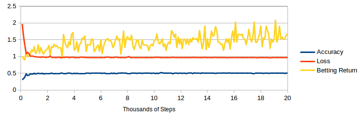
The above graph shows how the model developed as it was trained. The DNN converges quickly on a solution and achieves an accuracy of 51%. This accuracy is slightly below the performance of Bookmakers, Bet365 achieves around 53-54% on the same results.
The betting return is less stable, and is in the region of a 50% return on investment. This strategy simulation placed 35 bets whilst considering 172 possible matches. It is difficult to generate an accurate betting return figure, as the strategy places a statistically small number of bets and there is not much test data.
The odds used were only from Bet365, and further gains could probably be achieved by shopping around. That said, Bet365 often provided the most competitive odds available in the dataset.
If you would like to learn more about machine learning, I can highly recommend Stanford University - Machine Learning by Andrew Ng. I am about halfway through the course at the time of writing, and thoroughly appreciating its bottom up approach to these subjects.
You may also be interested in my previous article on object detection and recognition in images with TensorFlow.